Introduction
I came across a study (on the internet, not peer reviewed) that had the goal of evaluating how long coffee beans should rest after they’re roasted before they’re ground and tasted for quality. The full study report is here: https://cafekreyol.com/research/post-roast-rest-study/. For a little background, when coffee beans are roasted, CO2 gets trapped in the beans, and then escapes over time as the coffee beans rest. It is generally well accepted that coffee beans need to rest at least 24 hours, since the amount of CO2 in the beans right after roasting prevents the coffee from tasting as good as it can. However, after a certain number of days, the coffee will begin to taste stale.
When assessing roasted bean quality, the industry standard is to let coffee beans roast for about 24 hours. This study wanted to see if quality improved with an even longer rest time.
Study Design
I thought this study was very nicely designed (although I will discuss at the end on how I think it could potentially be improved). On day 0, they roasted 21 different coffee beans. They used a roaster that produced identical roasts for each of the beans, and they roasted each coffee 5 times. After this roasting, they had 105 (21 times 5) bags of coffee. The idea is that they would taste (cup) each of the coffees on days 4, 8, 11, 17, and 22 post-roast. One day before each tasting (days 3, 7, 10, 16, and 21), they roasted each of the coffees again, so that they could have a 24-hour rested control sample for each coffee and tasting.
The tasting was extremely standardized (down to water temperature and grind size), and each cup was blindly tasted by 3 expert raters. Each rater evaluated the coffee using a standardized scale (https://atlanticspecialtycoffee.com/wp-content/uploads/SCAA-Official-Cupping-Form.pdf), with a potential score between 0-100. However, cupping scores are usually between 80-95. The study has only publicly posted the average score for each coffee across the 3 raters.
Study Analysis
I think it is helpful to visualize the study data to get a better handle on what it looks like. I’m not going to go into data cleaning, although you can see how I did it using this github link.
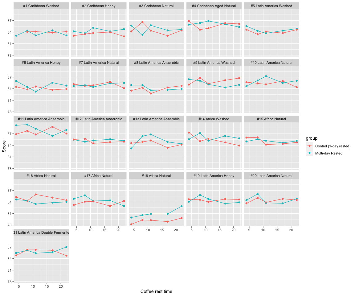
You can see that each coffee was tasting twice at each tasting. For each of the coffees, one of the cups had brewed coffee that had been roasted on day 0 (the “Multi-day Rested” in blue), and the other cup had brewed coffee that had been roasted 24-hours previously (the “Control (1-day rested)” in red.) Note that for Coffee #1, the 4-day rested coffee was not evaluated because there was a defect unrelated to the rest-time. I think this plot emphasizes the paired nature of each tasting, in that we can compare the rested coffee at each time point to a control sample that had been roasted 1-day before, but was (blindly) tasted at the same time.
The original study analysis proceeded as follows. First, they averaged the control sample scores for each coffee across each of the 5 tastings, rather than comparing the treatment (more resting time) coffee to the control coffee within each tasting. I find this interesting, as it seems that they set-up having 1-day rested coffees for each day to serve as an internal control, but then totally ignored this in the analysis (more on this later). For each coffee, they noted which day had the highest score, with the day 1 score being the average of all the roasted coffees. For each day they calculated the percentage of coffees where the beans with that rest time had the highest score, and they compared these percentages across days, finding that the majority of the 68% of the coffees peaked on either day 4, 8, or 11.
While this analysis is not totally unreasonable, especially for a non-academic study, statisticians have shown that its preferable to not dichotimize the data before doing the analysis–that is, by reducing each coffee to saying which day it peaked, rather than looking at the magnitude of the peak, we lose a lot of information.
For our first analysis, we will ignore the paired nature of the rested and control beans, and treat all of the control coffees as if they were tasted on day 1, since each of the controls were only tasted 1 day after they were roasted. This is essentially what the original analysis did. We can visualize this assumption and compare it to the study design plotted above.
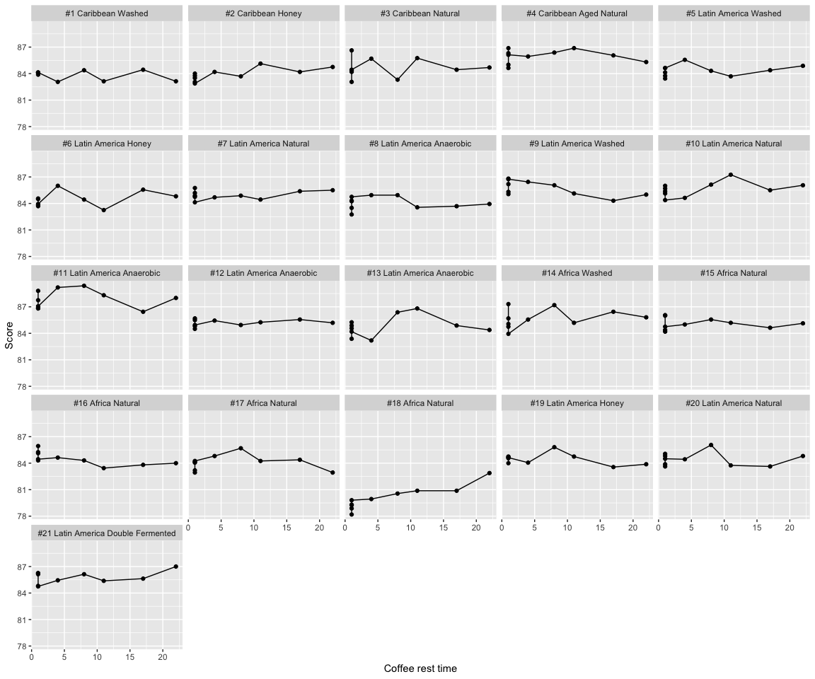
We see that this treats the data as if there were 5 scores for the 1-day rested beans, and then 1 score for the multi-day rested beans, for each coffee. To analyze this, we will use a random-intercept model, where each coffee gets a random intercept, and then each rest-day is a fixed effect. By using a random intercept model, we are saying that each coffee has its own baseline (day-1) score–some coffees are better than others, of course–but then we expect each of the changes from that baseline, due to rest time and tasting session, to be the same for all of the coffees. Here is how we would fit that model in R, and then show the estimates, standard errors, p-values, and 95% confidence intervals for our coefficients of interest.
library(lme4)
library(lmerTest)
library(emmeans)

### Show what data looks like
head(d_long_unpaired, 10)
## # A tibble: 10 × 6
##    coffee              group                    day score number day_factor
##    <fct>               <fct>                  <dbl> <dbl>  <dbl> <fct>
##  1 #1 Caribbean Washed Multi-day Rested           4  83.1      1 4
##  2 #1 Caribbean Washed Multi-day Rested           8  84.4      1 8
##  3 #1 Caribbean Washed Multi-day Rested          11  83.1      1 11
##  4 #1 Caribbean Washed Multi-day Rested          17  84.4      1 17
##  5 #1 Caribbean Washed Multi-day Rested          22  83.1      1 22
##  6 #1 Caribbean Washed Control (1-day rested)     1  NA        1 1
##  7 #1 Caribbean Washed Control (1-day rested)     1  84.1      1 1
##  8 #1 Caribbean Washed Control (1-day rested)     1  84.1      1 1
##  9 #1 Caribbean Washed Control (1-day rested)     1  83.9      1 1
## 10 #1 Caribbean Washed Control (1-day rested)     1  84.1      1 1
unpaired_model <- lmer(score ~ day_factor + (1 |coffee), data = d_long_unpaired)
coef_table <- coef(summary(unpaired_model))[,-c(3:4)]
coef_table <- cbind(coef_table,confint(unpaired_model)[-(1:2),] )
| Estimate | Std. Error | Pr(>|t|) | 2.5 % | 97.5 % | |
|---|---|---|---|---|---|
| (Intercept) | 84.57 | 0.31 | 0.00 | 83.94 | 85.20 |
| day_factor4 | 0.33 | 0.19 | 0.09 | -0.05 | 0.71 |
| day_factor8 | 0.70 | 0.19 | 0.00 | 0.32 | 1.07 |
| day_factor11 | 0.26 | 0.19 | 0.18 | -0.12 | 0.64 |
| day_factor17 | 0.09 | 0.19 | 0.65 | -0.29 | 0.47 |
| day_factor22 | 0.29 | 0.19 | 0.13 | -0.08 | 0.67 |
In the table above, the intercept represents the mean score for coffees that have been
rested for 1 day. day_factor4 represents the average difference in cupping
score for coffees that have been rested for 4 days vs 1 day, day_factor8 represents the average difference in cupping score for coffees that have been rested for 8 days vs 1 day, and the rest of the coefficients are interpreted similarly. We see
that this model finds a significant increase in cupping scores for coffees
that have been rested for 8 days vs 1 (estimated increase of .70, 95% CI of (.32, 1.07)), and does not find evidence that the cupping scores increases for other
days of rest. This is what was suggested in the original study, but now we come to this
conclusion through more a rigorous analysis that also gives us an effect size estimate.
We will now run an analysis which takes into account the paired nature of the tastings. This model will have a random intercept for each coffee, as before, but now our model will estimate the average control score for each tasting, as well as the average difference between the rested coffee and the control coffee at each tasting. This is essentially subtracting the rested beans and control beans score for each coffee, and estimating the mean for this at each tasting. As opposed to our first analysis, this analysis importantly does not assume that the scores for the control coffees tasted on one day can be switched for the scores of the control coffees tasted on another day–you might recognize this as not assuming exchangeability between control samples. This also importantly assumes that on average, each of the control coffees experience the same shift in scores within a tasting, which could happen from tasters on one day perhaps all giving higher scores than on another day.
### Show what data looks like
head(d_long_paired, 10)
## # A tibble: 10 × 6
##    coffee              group                    day score number day_factor
##    <fct>               <fct>                  <dbl> <dbl>  <dbl> <fct>
##  1 #1 Caribbean Washed Multi-day Rested           4  83.1      1 4
##  2 #1 Caribbean Washed Multi-day Rested           8  84.4      1 8
##  3 #1 Caribbean Washed Multi-day Rested          11  83.1      1 11
##  4 #1 Caribbean Washed Multi-day Rested          17  84.4      1 17
##  5 #1 Caribbean Washed Multi-day Rested          22  83.1      1 22
##  6 #1 Caribbean Washed Control (1-day rested)     4  NA        1 4
##  7 #1 Caribbean Washed Control (1-day rested)     8  84.1      1 8
##  8 #1 Caribbean Washed Control (1-day rested)    11  84.1      1 11
##  9 #1 Caribbean Washed Control (1-day rested)    17  83.9      1 17
## 10 #1 Caribbean Washed Control (1-day rested)    22  84.1      1 22
paired_model <- lmer(score ~ group*day_factor + (1 |coffee), data = d_long_paired)
coef_table <- coef(summary(paired_model))[,-c(3:4)]
coef_table <- cbind(coef_table,confint(paired_model)[-(1:2),] )
| Estimate | Std. Error | Pr(>|t|) | 2.5 % | 97.5 % | |
|---|---|---|---|---|---|
| (Intercept) | 84.59 | 0.35 | 0.00 | 83.89 | 85.29 |
| groupMulti-day Rested | 0.31 | 0.25 | 0.23 | -0.18 | 0.80 |
| day_factor8 | 0.18 | 0.25 | 0.47 | -0.31 | 0.67 |
| day_factor11 | -0.12 | 0.25 | 0.64 | -0.61 | 0.37 |
| day_factor17 | -0.03 | 0.25 | 0.90 | -0.52 | 0.46 |
| day_factor22 | -0.14 | 0.25 | 0.58 | -0.63 | 0.35 |
| groupMulti-day Rested:day_factor8 | 0.18 | 0.36 | 0.61 | -0.51 | 0.87 |
| groupMulti-day Rested:day_factor11 | 0.05 | 0.36 | 0.89 | -0.64 | 0.74 |
| groupMulti-day Rested:day_factor17 | -0.21 | 0.36 | 0.56 | -0.90 | 0.48 |
| groupMulti-day Rested:day_factor22 | 0.11 | 0.36 | 0.77 | -0.58 | 0.79 |
The coefficient interpretation is now different. The groupRested
coefficient estimates the average difference in tasting scores between
4-day rested coffees and 1-day rested coffees. day_factor8, day_factor11,
day_factor17, and day_factor22 estimate the average difference in control
cupping scores comparing days 8, 11, 17, and 22 to day 4, respectively. The complicated
part of this model is the interpretation of the interaction effects. For example,
the groupRested:day_factor8, coefficient estimates
the difference between the differences of coffees rested 8 days compared to 1 day vs
coffees rested 4 days compared to 1 day. To get the the we actually want–
the differences between coffees rested 8, 11, 17, and 22 days vs 1 day–
we can use the emmeans package.
contrasts <- emmeans(paired_model, specs = pairwise ~ group|day_factor, type = "response")$contrasts
| contrast | day_factor | estimate | SE | df | t.ratio | p.value |
|---|---|---|---|---|---|---|
| (Control (1-day rested)) - (Multi-day Rested) | 4 | -0.3067079 | 0.2548417 | 179.0353 | -1.2035231 | 0.2303629 |
| (Control (1-day rested)) - (Multi-day Rested) | 8 | -0.4895238 | 0.2513840 | 179.0000 | -1.9473149 | 0.0530616 |
| (Control (1-day rested)) - (Multi-day Rested) | 11 | -0.3571429 | 0.2513840 | 179.0000 | -1.4207064 | 0.1571417 |
| (Control (1-day rested)) - (Multi-day Rested) | 17 | -0.0990476 | 0.2513840 | 179.0000 | -0.3940092 | 0.6940432 |
| (Control (1-day rested)) - (Multi-day Rested) | 22 | -0.4123810 | 0.2513840 | 179.0000 | -1.6404423 | 0.1026693 |
While the emmeans package flips the comparisons around (i.e. a negative number means a higher score for multi-day rested coffees), we see again that we still estimate that coffees rested 8 days have the higher score. However, the estimated difference is now lower than when we did the unpaired analysis, and the p-value is just above the .05 significance level. Thus we this analysis does not allow us to conclude that there is a significant effect of resting coffee for more than 1-day, although I would not be surprised to see if a slightly larger future study were to find this out. In addition, this analysis does not show that there was a “tasting” effect, as the average score of the control coffees were similar across each tasting session.
Conclusion and Recommendations for Future Studies
I thought this was a really nicely designed study. The authors clearly thought carefully about controlling all factors that might contribute to variable cupping scores, which is more than you can say about most experimental designs. The conclusion from a statistical analysis depends on what you’re willing to assume about exchangability of control sample scores across the different days. If you ignore the fact that each control coffee was scored on a different day, in conjunction with a multi-day rested coffee, then you see some evidence that resting coffees does result in higher cupping scores. However, we fail to see that if we take into account the paired nature of the experiment.
If this experiment were to be repeated, I would change the design just a bit. Rather than roasting all coffees on day 0, and then doing 5 different tastings, I would only have 1 tasting (if possible). I would then do 6 different roast sessions–one 22 days before, one 17 days before, one 11 days before, one 8 days before, one 4 days before, and one 1 day before. Then for each coffee and rest-time, I would have multiple samples to be evaluated. Because the roasting is more controlled than the cupping, this eliminates the variability of each cupping being performed on different days, so we don’t have to make as many assumptions for the analysis.
Of course, there are other ways you could analyze this data, so I’d be interested to see what other people recommend and conclude–I expect that some people would want to do a Bayesian analysis. I think this is a great dataset for teaching as well, since it teaches about experimental design, the importance of assumptions in analysis, coefficient interpretation, and random effects.