This past week’s NFL divisional playoff round was probably the best weekend of football that I can remember watching, with twists and turns in every game, and the weekend concluding with the Chiefs and Bills having a record setting last two minutes. However, as many statisticians know, feelings don’t always match reality. I wanted to use NFL win probability data from games during this season to see if this weekend’s playoff games were as wild as I felt they were.
Luckily, the nflfastR package makes it incredibly easy to collect data and get predicted win probabilities throughout each game, using their model trained using xgboost. There is also public code generously provided by Geoffrey Grosenbach to help us prepare the data for the model.
We will first load the necessary libraries and download the data. Note you can change the year to any year (until 1999) if you want to collect more data. This data contains information on every play of the NFL season!
library(nflfastR)
library(tidyverse)

year <- 2021
url = str_interp(
    "https://raw.githubusercontent.com/guga31bb/nflfastR-data/master/data/play_by_play_${year}.rds"
)
win_prob_dir <- 'win_prob_data'
if(!dir.exists(win_prob_dir)) {
    dir.create(win_prob_dir)
}
local_filename = str_interp(file.path(win_prob_dir, "play_by_play_${year}.rds"))
if (!file.exists(local_filename)) {
    download.file(url, local_filename)
}
We can then read in the play-by-play data from 2021, create an indictor for whether the home team is the team that is on offense for a given play (posteam). We do this because the model will give us the win probability for the team that’s on offense, but we will need to convert this into the win probability for the home team.
wp_data <-
    readRDS(str_interp(file.path(win_prob_dir, "play_by_play_${year}.rds"))) %>%
    dplyr::mutate(
        # create home indicator used in model
        home = ifelse(posteam == home_team, 1, 0)
    ) %>%
    # creates Diff_Time_Ratio and spread_time
    nflfastR:::prepare_wp_data()
We will then select the columns needed for the win probability model to give us our predictions, filter out plays which have missing data that will affect the win probability predictions, as well as excluding overtime plays. We feed this data into the nflfastR function calculate_win_probability, which will add a the win probability to our data as a column titled wp. We finally will transform the win probability for the team on offense to the win probability for the home team.
cols_for_wp <- c("game_id", "receive_2h_ko", "score_differential", "home_team", "posteam",
                 "half_seconds_remaining", "game_seconds_remaining",
                 "spread_line", "down", "ydstogo", "yardline_100", "posteam_timeouts_remaining",
                 "defteam_timeouts_remaining")
wp_2021 <-
    wp_data %>%
    filter(
        !is.na(score_differential),
        !is.na(play_type),
        !is.na(down),
        !is.na(yardline_100),
        !is.na(defteam_timeouts_remaining),
        !is.na(posteam_timeouts_remaining),
        qtr <= 4
    ) %>%
    select(all_of(cols_for_wp)) %>%
    nflfastR::calculate_win_probability() %>%
    mutate(home_team_wp = ifelse(posteam == home_team, wp, 1- wp))
There are several metrics which one could think of to see which games are the most exciting (or volatile). I will use a simple metric of calculating the average change in (absolute) win probability across each play for the home team in each game. Games that are exciting, with lots of back-and-forth scoring (especially at the end of games), should rank highly on this metric.
I first arrange the data by game, and then descending from first play to last. For each play of the game (excluding the first play), we can use the lag function to create a variable that gives us the win probability for the home team from the previous play. Finally, we create our average change in win probability from each play over the course of game variable (mean_change) and arrange the games from most volatile to least.
wp_2021_mean_change <-
    wp_2021 %>%
    arrange(game_id, -game_seconds_remaining) %>%
    group_by(game_id) %>%
    mutate(wp_lag = lag(home_team_wp, order_by=game_id)) %>%
    filter(!is.na(wp_lag)) %>%
    summarise(mean_change = mean(abs(home_team_wp - wp_lag)))%>%
    arrange(desc(mean_change))
We can now see what the 5 most volatile games of the 2021 season were.
most_volatile_games <- wp_2021_mean_change$game_id[1:5]
most_volatile_games
## [1] "2021_20_BUF_KC"  "2021_06_DAL_NE"  "2021_11_BAL_CHI" "2021_02_MIN_ARI"
## [5] "2021_06_BUF_TEN"
Unsurprisingly, the Chiefs vs Bills game ranked number one, showing us that this is a reasonable metric. We will write a function to plot the win probability for games of interest.
plot_win_prob <- function(wp_data = wp_2021, game, ylab) {
    wp_2021 %>%
    mutate(minutes_left_in_game = game_seconds_remaining / 60) %>%
    filter(game_id == game) %>%
    ggplot(aes(x = minutes_left_in_game, y = home_team_wp)) +
    geom_line(alpha = .5) +
    scale_x_reverse() +
    scale_y_continuous(breaks = c(0, .25, .5, .75, 1),
                       limits = c(0, 1)) +
    labs(x = "Minutes left in regulation time", y = ylab)
}
plot_win_prob(game = "2021_20_BUF_KC", ylab = "KC Win Probability")
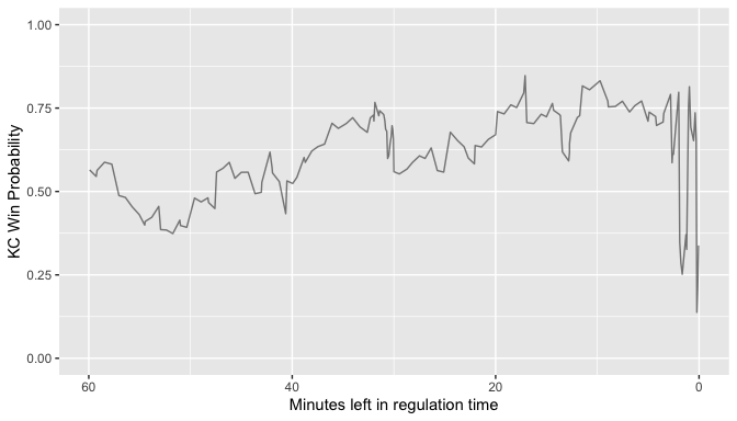
Interestingly, we see that the win probability just before over time was still under 50%, because the last win probabilities were before they made the field goal to tie the game.
We can also look at the other four games:
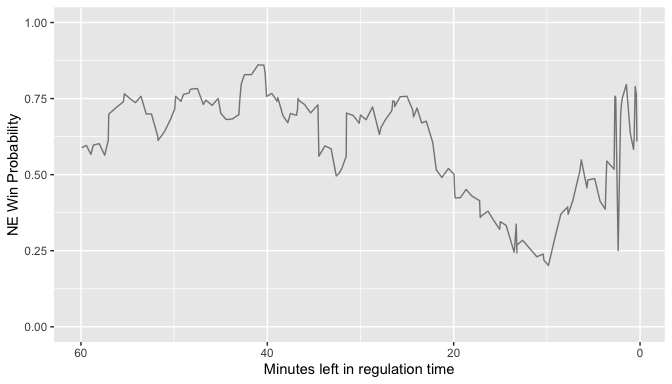
- Week 6 Dallas at New England: New England was up 21-20 with 2:42 left in the game, with Dallas just having missed a field goal. Dallas then gets a pick-6, which is immediately followed by a 75 yard touchdown pass by New England to go up by 3. Dallas then has a 9 drive play in under 2 minutes to send the game to overtime.
plot_win_prob(game = "2021_06_DAL_NE", ylab = "NE Win Probability")
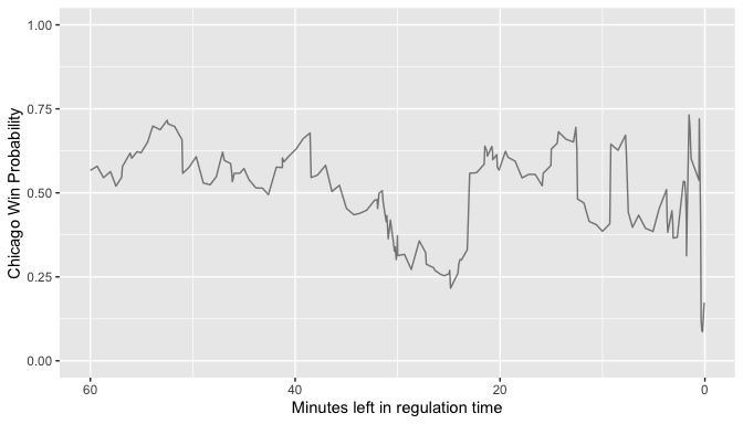
- Week 11 Baltimore at Chicago:. Baltimore kicks a field goal to go up 9-7 with less than 4 minutes to go. Chicago drives down with a 10-play, 75 yard drive in 2 minutes to go up 13-9, only to end up giving up a 5-play, 72 yard drive in 1 minute and 20 seconds to lose the game 16-13.
plot_win_prob(game = "2021_11_BAL_CHI", ylab = "Chicago Win Probability")
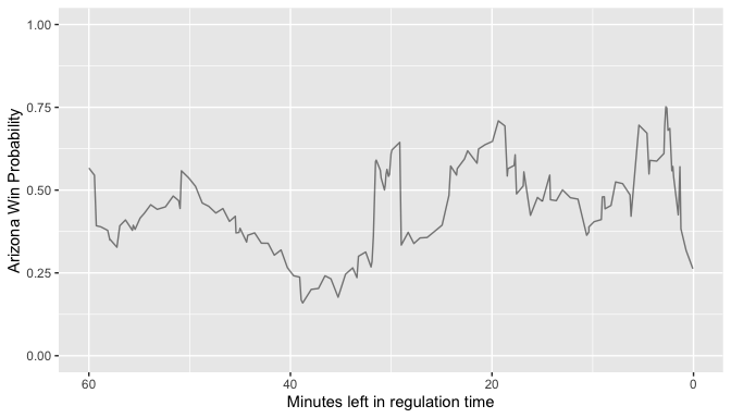
- Week 2 Minnesota at Arizona:. The recap headline on ESPN says it all: “Cards win 34-33 thriller after Vikings miss last-second FG”. Minnesota went from being up 20-7 partway through the 2nd quarter, only to be down 24-23 at half. The 2nd half was a much more defensive game, but Minnesota had the opportunity to win it with an easy 37-yard field goal at the end, which resulted in Arizona having a low win probability on the last play of the game (shown below). However, Minnesota missed the kick and lost the game.
plot_win_prob(game = "2021_02_MIN_ARI", ylab = "Arizona Win Probability")
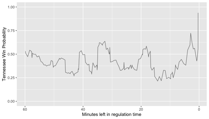
- Week 6 Buffalo at Tennessee:. The headline again tells us how exciting this game was: “Titans stop Allen on 4th down, hang on to beat Bills 34-31”. Buffalo was leading almost the whole game, until Tennessee took a 34-31 lead with 3:05 left in the game. Buffalo stormed down the field to set up a 1st & 10 from the Tennessee 12-yard line with 50 seconds to go, giving them a win probability of over 50%. However, Tennessee ended up with a goal-line stand and the win.
plot_win_prob(game = "2021_06_BUF_TEN", ylab = "Tennessee Win Probability")
Thanks for reading–it would be great to hear if you have other ideas for metrics that better capture game volatility. It would definitely be interesting to look back further and see what the most volatile games of the past 20 seasons have been, to see if the Chiefs vs Bills game stands up.