Recently I’ve been studying about identifying structural variants using short NGS reads. I don’t want to go into detail about structural variants (for more information you can read the Wikipedia page), but I want to briefly show how you can visualize genomic deletions in R with short reads.
In a deletion event, a portion of the DNA that is included in the reference is deleted from the genome of interest. Short reads can help us find deletion regions, due to our knowledge of what the “insert size” of the DNA fragments should be. To understand what insert size is, we first have to get a sense of how these short reads are generated. The DNA sequence of interest first starts off as a collection of very long strands. Wet lab members then using shearing techniques to break the DNA into short fragments, usually around 700 basepairs (bp) or so in size, depending on the shearing technique. Finally, a common sequencing technique called read pair sequencing is used. The sequencer collects the DNA sequence of 150 bp reads from both sides of the fragment. These two reads put together are called a fragment, and we know that the size (in basepairs) between the end of the first fragment and the beginning of the second fragment should be around 400 bp. This might be more easily visualized in the following manner:
R1S—-R1E———————R2S—-R2E
Using R1S and R1E (and R2S and R2E) denote the start and end of the first (and second) read, we know the distance between R1S and R1E (and R2S and R2E) is 150 bp, and the distance between R1S and R2E is the fragment size, which is 700 bp. Thus, the distance between R1E and R2S, the insertion size, must be 400 bp.
Knowing that pairs of reads must be around 400 bp from each other helps alignment algorithms in determining where these reads align to the reference genome. However, if there is a deletion event in a given region, there isn’t DNA from this portion of the reference genome to be sequenced and thus mapped back to the reference. Thus, for reads in the deletion region, the R1 reads will be mapped to the left of the region in the reference genome, and the R2 reads will be mapped to the right of the region in the reference genome, leaving an empty gap of no reads mapping to the deletion region. Furthermore, we can keep track of which reads are pairs, and we can calculate their insert size. If the reads span the deletion region, and the region is significantly larger than 400 bp, the insert size will appear much larger than 400 bp, even though we know this cannot be true since the reads came from the same 700 bp fragment! This allows us to search read pairs for large insert sizes to identify potential deletion regions.
To visualize what I’ve described above, we’ll use a publically available BAM file. BAM files are the file format for containing mapped sequence reads. The BAM file is available under Data at this site. I will use wget, a command line tool, to download the data. Here is the code I used, although feel free to download the BAM file however you want. This will download the BAM file to the bam-files directory, and took about 8 minutes on my laptop.
mkdir -p bam-files
cd bam-files
wget "http://content.cruk.cam.ac.uk/bioinformatics/CourseData/IntroToIGV/HCC1143.normal.21.19M-20M.bam"
Now we will move to R. First we will download the necessary packages from Bioconductor.
source("https://bioconductor.org/biocLite.R")
biocLite("GenomicRanges")
biocLite("GenomicAlignments")
biocLite("ggbio")
biocLite("Rsamtools")
Because I already know the region where the deletion is, I can specify this region in R using a GenomicRanges object. For more on GenomicRanges, I highly recommend reading Kasper Hansen’s guide. Here, my region of interest is in chromosome 21 (whether it’s written 21 or chr21 depends on the reference genome), and I’m interested in bases 19326000-19330000. The autoplot function, from the ggbio package, does quite a lot in this one function call. It extracts all short reads from the BAM file that overlap with my region of interest, determines which ones are paired, and uses ggplot2 to plot the short reads (larger black rectangles), with read pairs connected by a line. The x-axis shows where in chromosome 21 we are, in basepairs, relative to the start.
library(GenomicRanges)
library(ggbio)
library(Rsamtools)
region.interest <- GRanges("21", IRanges(start = 19326000, end = 19330000))
bamfile <- file.path("bam-files", "HCC1143.normal.21.19M-20M.bam")
indexBam(bamfile)
##       bam-files/HCC1143.normal.21.19M-20M.bam
## "bam-files/HCC1143.normal.21.19M-20M.bam.bai"
autoplot(bamfile, which = region.interest, geom = "gapped.pair")
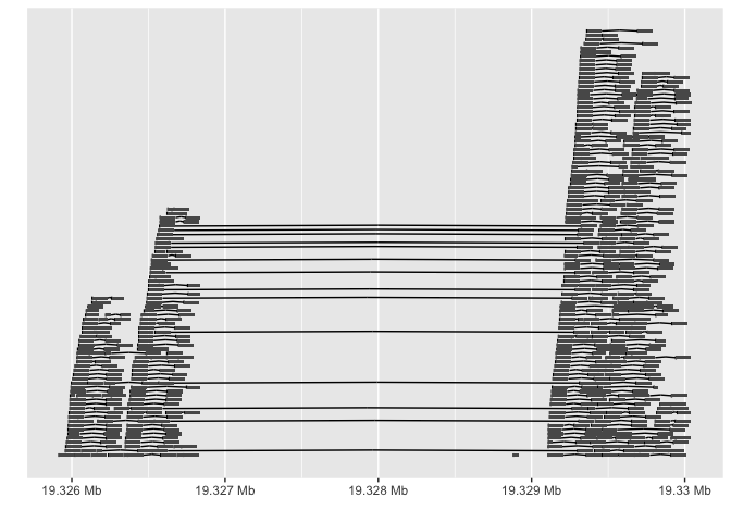
We can see that between 19327000 and 19329000 basepairs there are no reads, and only long lines connecting read pairs. Because these long lines represent the inserts between read pairs, and they’re over 2000 bp long (significantly larger than the insert size between read pairs outside of this region), we see a clear deletion!
While this is just one type of structural variation, I hope this post helps clarify how you can easily visualize structural variants in R, either for verification of software results, or for exploration. If you have other ways of visualizing structural variants in R, please share via twitter, email, or the comments section.